Theory, Made Useful Explainer 1 - If a Decision Tree Falls in a Random Forest and no One is Around to Hear - Did it Make a Sound?

On trees, forests, and the noise between them

Part of the “Theory, Made Useful” Series - Explainer 1

What role does a single decision tree play inside a random forest? Does it matter on its own, or only as part of the collective?

In this article, we’ll cover:

• Decision trees, in plain words: how splits work (Gini/Entropy), why they overfit, and a quick baseline on our dataset.
• Taming a tree: pruning (cost-complexity) and growth limits (max_depth, min_samples_*) with before/after results.
• Random Forest = bagging + random features: why averaging many decorrelated trees helps - the forest swallows the noise of a single overfitted tree - plus OOB as a built-in check.
• From forest to insight: SHAP summary/beeswarm to see which features matter and in what direction.
• Practical takeaways: when to prefer a single interpretable tree, when to deploy a forest, and how to report metrics cleanly.

Important disclaimer: The data set used in this article is a synthetic data set, created for model explanation only. The trees are imaginary, the rainfall obeys a random number generator, and the sunlight was rounded for your convenience. Do not use this as botany or forestry guidance - no planting, pruning, logging, or squirrel-rehoming decisions should be based on it. No trees were harmed in this analysis - some were merely overfitted.

---

Decision Trees: How They Work?

Decision trees are versatile models that can handle both classification and regression tasks. They make predictions by recursively splitting the dataset into smaller, more homogeneous subsets, following a hierarchical “if-then” structure.

How does a decision tree decide where to split?

At each step, the algorithm evaluates every available feature and chooses the best split according to a criterion. The two most common criteria for classification are:

• Gini Impurity - measures how often a randomly chosen sample would be misclassified if it were labeled according to the distribution in the node.
• Entropy (Information Gain) - measures the amount of uncertainty (disorder) in the node, and how much uncertainty is reduced after the split.

For regression tasks, the usual criterion is variance reduction (how much the split reduces the spread of the target values).

The process in action

1. Evaluate all features and thresholds - compute the impurity measure for each possible split.
2. Choose the split that reduces impurity the most - the one that makes the resulting subsets as homogeneous as possible.
3. Create new nodes from these subsets.
4. Repeat recursively until a stopping condition is met (e.g., maximum depth, minimum samples, or pure leaves).

The result is a tree where the root node represents the strongest discriminator, and subsequent branches capture finer distinctions.

Here is a simplified version of our decision tree (pruned, reduced depth just for visualization)

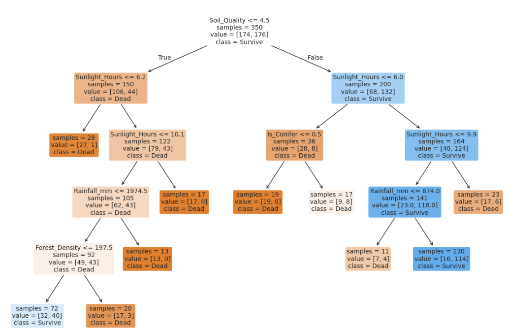
What does this tree shout at us?

Root Node: Soil Quality is the most important discriminator: poor soil leans toward Dead, better soil leans toward Survive. What is poor? ≤4.5

Left branch (Soil ≤ 4.5): If Sunlight ≤ 6.2 hours the trees death rate is high, if sunlight > 6.2 and < 10.1 death rate is lower but still high. If sunlight > 10.1 then Rainfall becomes critical, as if it is more than 1,975mm survival drops again. If it is less than 1,975mm, then forest density is critical. Below 197.5 trees per hectare, the majority survive, and above 197.5 trees per hectare, the majority dies.

Summary: Poor soil + too little/too much sunlight + excess dense forests + rain → mostly dead trees.

This is an analysis of a limited depth. As we learned, these splits repeat recursively. If no stopping condition is set, the tree will keep growing until it perfectly memorizes the training data, reaching 100% accuracy. Although we can set limits, this already hints at the main problem with single decision trees: overfitting.

Let’s have a look at our dataset:

import pandas as pd
import matplotlib.pyplot as plt
import seaborn as sns

from sklearn.model_selection import train_test_split
from sklearn.tree import DecisionTreeClassifier
from sklearn.metrics import classification_report, confusion_matrix

# Get dummies
df = pd.get_dummies(data = df, columns = ['Leaf_Size'])

# Separating the target variable and other variables
Y = df.Survival_in_Forest
X = df.drop(['Survival_in_Forest'], axis = 1)

# split the data
X_train, X_test, y_train, y_test = train_test_split(X, Y, test_size = 0.3, random_state = 90210)

# Building decision tree model
dt = DecisionTreeClassifier(class_weight="balanced", random_state=90210)
dt.fit(X_train, y_train)

# Checking performance on the training dataset
y_train_pred_dt = dt.predict(X_train)
def metrics_score(actual, predicted):
   print(classification_report(actual, predicted))
   cm = confusion_matrix(actual, predicted)
   plt.figure(figsize = (8, 5))
   sns.heatmap(cm, annot = True, fmt = ".0f", linewidths = 0.5, square = True, cmap = "PiYG")
   plt.ylabel("Actual label")
   plt.xlabel("Predicted label")
   plt.title("Confusion Matrix")
   plt.show()
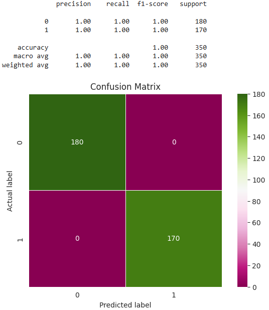
metrics_score(y_train, y_train_pred_dt)

And the results are suspiciously perfect:

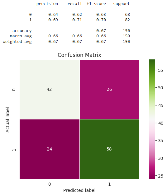
Let’s see what going on on the test:

y_test_pred_dt = dt.predict(X_test)

metrics_score(y_test, y_test_pred_dt)

Can we mitigate this overfitting?

One excellent - though not perfect - way to handle overly complex decision trees is pruning. Pruning adds a penalty for branching: we set a parameter α (alpha, the cost-complexity parameter) that determines the tradeoff between tree size and training error. If a split does not reduce the error enough to offset the added complexity, the branch is cut back. This reduces the tree’s complexity and prevents it from fitting the training set too perfectly.

Let’s prune

import numpy as np
import matplotlib.pyplot as plt
from sklearn.model_selection import cross_val_score
from sklearn.tree import DecisionTreeClassifier

# 1) Get the effective alphas for cost-complexity pruning
#     cost_complexity_pruning_path() gives back possible values of ccp_alpha
#     each alpha corresponds to pruning away some branches

path = dt.cost_complexity_pruning_path(X, Y)

# 2) Sample 25 possible pruning strengths (ccp_alpha values)
#    between the smallest and largest suggested by the path
alphas = np.linspace(path.ccp_alphas.min(), path.ccp_alphas.max(), 25)

scores = []
for a in alphas:
# 3) For each alpha, train a pruned decision tree
#     ccp_alpha controls the pruning penalty
#     min_samples_leaf=5 ensures leaves have at least 5 samples
    m = DecisionTreeClassifier(random_state=90210, ccp_alpha=a, min_samples_leaf=5)
    s = cross_val_score(m, X, Y, cv=5, scoring="f1")

# 4) Evaluate the model with 5-fold cross-validation using F1-score
    scores.append(s.mean())

# 5) Select the alpha that produced the best average cross-validated F1 score
best_alpha = alphas[np.argmax(scores)]

# 6) Train the final pruned decision tree with the chosen alpha
dt_pruned = DecisionTreeClassifier(
    random_state=90210,
    ccp_alpha=best_alpha,
    min_samples_leaf=5
).fit(X, Y)

# Plot Cost-Complexity Pruning Path

plt.figure(figsize=(7,4))
plt.plot(alphas, scores, marker="o")
plt.axvline(best_alpha, ls="--", lw=1)
plt.xlabel("ccp_alpha")
plt.ylabel("CV F1 (mean, 5-fold)")
plt.title("Cost-Complexity Pruning Path")
plt.show()
print("Best alpha:", best_alpha)

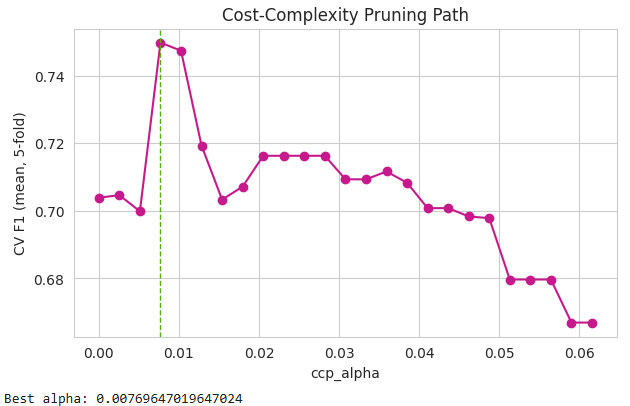
How to read this?

• The x-axis = pruning strength (α)
• The y-axis = mean F1 score from 5-fold cross-validation on the training set
• The green dashed line = best α, in this case ~ 0.77

Interpretation

• Small α (left side): Tree is very complex, with many branches - high variance, risk of overfitting.
• Large α (right side): Tree is overly simplified - high bias, underfitting.
• Sweet spot: Around α = 0.77, where the tree balances complexity and generalization.

Let’s see how our pruned tree model performs:

# 4) Fit final model on TRAIN
dt_pruned = DecisionTreeClassifier(
    random_state=90210,
    ccp_alpha=best_alpha,
    min_samples_leaf=5
)
dt_pruned.fit(X_train, y_train)

# 5) Train metrics
y_pred_tr = dt_pruned.predict(X_train)
print("*** TRAIN REPORT ***")
print(classification_report(y_train, y_pred_tr, target_names=["Dead","Survive"]))
print("TRAIN Confusion:\n", confusion_matrix(y_train, y_pred_tr))

# 6) Test metrics
y_pred_te = dt_pruned.predict(X_test)
y_proba_te = dt_pruned.predict_proba(X_test)[:, 1]
print("\n*** TEST REPORT ***")
print(classification_report(y_test, y_pred_te, target_names=["Dead","Survive"]))
print("TEST Confusion:\n", confusion_matrix(y_test, y_pred_te))

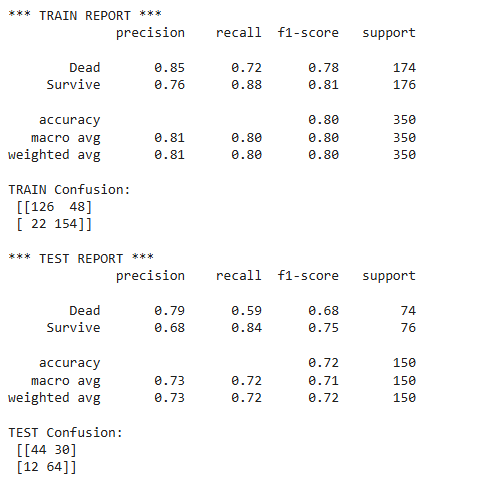
Results & Conclusion

• The pruned tree performs better than the unpruned one - it reduces noise and overfitting.
• However, even after pruning, a single decision tree still tends to overfit and capture noise.

Another Way to Control Overfitting

Besides post-hoc pruning, we can also restrict the tree’s growth in advance through hyperparameters:

• max_depth - limits how deep the tree can grow.
• min_samples_leaf - enforces a minimum number of samples per leaf.
• min_samples_split - enforces a minimum number of samples per node in order to split.

Key difference from pruning:

• Pruning: Let the tree grow fully, then cut back unhelpful branches (based on cost complexity).
• Hyperparameter tuning: Impose size/shape rules from the start, without knowing ahead of time which branches are meaningful.

How to?

import numpy as np

from sklearn.tree import DecisionTreeClassifier
from sklearn.model_selection import GridSearchCV, train_test_split
from sklearn import metrics
from sklearn.metrics import (
    classification_report,
    confusion_matrix,
    recall_score,
    roc_auc_score
)

dtree_estimator = DecisionTreeClassifier(class_weight = 'balanced', random_state = 90210)

# Grid of parameters to choose from
parameters = {'max_depth': np.arange(2, 8),           # How deep the tree can grow
              'criterion': ['gini', 'entropy'],       # Data impurity criterion
              'min_samples_leaf': [5, 10, 20, 25, 30],# Minimum number of samples per leaf
              'min_samples_split': [2, 5, 10, 15, 20] # Minimum number of samples per node in order to split
             }

# Type of scoring used to compare parameter combinations
scorer = metrics.make_scorer(recall_score, pos_label = 1)

# Run the grid search 5-fold cross-validation
gridCV = GridSearchCV(dtree_estimator, parameters, scoring = scorer, cv = 5)

# Fitting the grid search on the train data
gridCV = gridCV.fit(X_train, y_train)

# Set the classifier to the best combination of parameters
dtree_estimator = gridCV.best_estimator_

# Fit the best estimator to the data
dtree_estimator.fit(X_train, y_train)

# ***( Train Metrics )***
print("*** TRAIN REPORT ***")
print(classification_report(y_train, y_pred_train, target_names=["Dead","Survive"]))
print("TRAIN Confusion:\n", confusion_matrix(y_train, y_pred_train))
print("TRAIN ROC-AUC:", roc_auc_score(y_train, y_proba_train).round(3))

# ***( Test Metrics )***
print("\n*** TEST REPORT ***")
print(classification_report(y_test, y_pred_test, target_names=["Dead","Survive"]))
print("TEST Confusion:\n", confusion_matrix(y_test, y_pred_test))
print("TEST ROC-AUC:", roc_auc_score(y_test, y_proba_test).round(3))

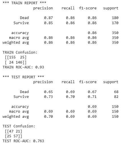
Results & Conclusion

• The hyperparameter-tuned tree performs better than the base model but worse than the pruned model

Decision Trees Strengths and Weaknesses

Strengths

• Interpretability: Decision trees are straightforward and intuitive. They provide clear, human-readable rules (e.g., If Sunlight ≤ 6.2 hours, the tree death rate is high).
• Ease of use: They require few assumptions, no complex preprocessing, and minimal scaling of features.
• Non-linearity: Decision trees can naturally capture non-linear relationships between variables.

Weaknesses

• Overfitting: They have a strong tendency to overfit, especially when grown deep without constraints.
• Instability: Small changes in the data can lead to very different splits and structures.

Random Forest

We’ve seen that a lone tree has overfitting and stability weaknesses. To deal with these weaknesses, we can use a technique that combines bootstrapping (resampling the dataset to create several datasets) and aggregating the results of these models into one stabilized result. This is called bagging - Bootstrap (B) + Aggregation (Agg).

One such bagging algorithm is Random Forest. A random forest is an ensemble of decision trees. Each tree is trained on a bootstrap resample of the rows and, at each split, is allowed to consider only a random subset of features (variables). So, whereas plain bagging uses a subset of the dataset (rows) but all features, random forests also sample the set of independent variables at each split.

The final prediction of the forest is the result of ensemble voting, with each tree casting a vote.

In random forests, we then have other important hyperparameters in our grid: max_features, which sets a limit to the maximum number of variables a split may consider and n_estimators: which sets the number of trees in the forest.

How does it help? A decision tree’s main problem is overfitting to noise. By sampling only a subset of features at each split (and bootstrapping rows), the overfitting of an extra-noisy tree - one that latched onto a noisy feature - is mitigated by the votes of quieter trees that didn’t train on that feature.

In other words, the forest swallows the noise of a single overfitted tree.

Do we hear the noise that the trees make?

Out-of-bag (OOB) error is the forest’s built-in way to check itself. Each tree is trained on a bootstrap sample, which leaves out about one-third of the samples (rows) for that tree. For each training row, we collect predictions only from the trees that never saw it, combine those (vote/average), and compare to the true label. The overall mismatch rate is the OOB error.

We can think of it as a cross-validation for free: an internal estimate of test error without touching our test set. If our training score is high but the OOB score lags, we’re overfitting. If they’re close, the ensemble is doing its job - the forest swallows the noise of a single overfitted tree.

(Notes: OOB works when bootstrap=True; in scikit-learn we’ll see it as oob_score_ on the fitted RandomForest.)

Random Forest - How to?

from sklearn.ensemble import RandomForestClassifier
from sklearn.model_selection import GridSearchCV
from sklearn.metrics import (
    classification_report, confusion_matrix, roc_auc_score, recall_score
)
import numpy as np
from sklearn import metrics

#  Estimator
rf_estimator = RandomForestClassifier(
    class_weight='balanced',
    random_state=90210,
    n_jobs=-1,
    bootstrap=True,
    oob_score=True  # out-of-bag validation
)

# Train/test split
X_train, X_test, y_train, y_test = train_test_split(
    X, Y, test_size=0.3, random_state=7, stratify=Y
)

# Grid of parameters
rf_params = {
    'n_estimators': [400, 600, 800], # Number of trees in the forest
    'max_depth': [6, 8, 10],         # How deep the tree can grow
    'min_samples_leaf': [3, 5, 10],  # Minimum number of samples per leaf
    'min_samples_split': [2, 5, 10], # Minimum number of samples per node in order to split
    'max_features': [2, 4, 6, 8]     # per-split feature subset
}

# coring (same idea: recall on class 1)
rf_scorer = metrics.make_scorer(recall_score, pos_label=1)

#  Grid search
rf_grid = GridSearchCV(
    rf_estimator,
    rf_params,
    scoring=rf_scorer,
    cv=5,
    n_jobs=-1,
    refit=True
)

rf_grid.fit(X_train, y_train)
rf_best = rf_grid.best_estimator_

#  Predictions/Probas
y_pred_train = rf_best.predict(X_train)
y_proba_train = rf_best.predict_proba(X_train)[:, 1]

y_pred_test  = rf_best.predict(X_test)
y_proba_test = rf_best.predict_proba(X_test)[:, 1]

#  Reports
print("*** BEST PARAMS ***")
print(rf_grid.best_params_)
if hasattr(rf_best, "oob_score_"):
    print("OOB score:", round(rf_best.oob_score_, 3))

print("\n*** TRAIN REPORT ***")
print(classification_report(y_train, y_pred_train, target_names=["Dead","Survive"]))
print("TRAIN Confusion:\n", confusion_matrix(y_train, y_pred_train))
print("TRAIN ROC-AUC:", roc_auc_score(y_train, y_proba_train).round(3))

print("\n*** TEST REPORT ***")
print(classification_report(y_test, y_pred_test, target_names=["Dead","Survive"]))
print("TEST Confusion:\n", confusion_matrix(y_test, y_pred_test))
print("TEST ROC-AUC:", roc_auc_score(y_test, y_proba_test).round(3))

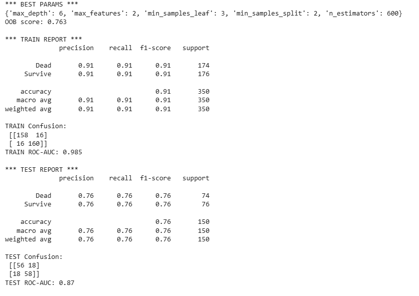
We can see how bagging and limiting features help: accuracy, AUC, precision, and recall all improved.

OOB accuracy ≈ test accuracy (0.763 vs. 0.76). That’s a solid internal check.

The train/test gap (0.91 → 0.76) is smaller than the tree’s gap; variance is down - the forest swallows the noise of a single overfitted tree.

What’s the trade-off?

Random Forest weaknesses

• Technical: Higher computational cost, more memory, and longer run time than a single tree.
• Interpretability: From a business/domain point of view, a single tree is easier to read. It gives clear if-then rules, explicit interactions, and numeric thresholds. A random forest - being a vote of many trees - doesn’t hand you one simple rulebook.

How do we extract business insight from a forest?

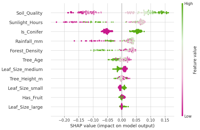
SHAP helps. The SHAP explainer assigns each feature a contribution to each prediction - how much that feature pushes the prediction up or down relative to a baseline. A SHAP summary plot ranks features by their average impact (mean absolute SHAP value). It won’t give the neat, human-readable rules a single tree provides, but it does show which variables matter most and in what direction - which is already useful.

import numpy as np
import shap
import matplotlib.pyplot as plt

import shap
from matplotlib.colors import LinearSegmentedColormap

cmap = LinearSegmentedColormap.from_list(
    'bubblegum_pistachio', ['#d01c8b', '#f2b4d4', '#d9f0d3', '#4dac26']
)

# ensure numeric inputs to SHAP
Xtr = X_train.astype(float)
Xte = X_test.astype(float)

explainer = shap.TreeExplainer(rf_best)
sv = explainer(Xte, check_additivity=False)

# pick the index of the positive class (label == 1)
pos_idx = int(np.where(rf_best.classes_ == 1)[0][0])

# reshape to single-output Explanation
if getattr(sv, "values", None) is not None and sv.values.ndim == 3:
    sv_pos = shap.Explanation(
        values        = sv.values[:, :, pos_idx],   # (n, features)
        base_values   = sv.base_values[:, pos_idx], # (n,)
        data          = sv.data,                    # (n, features)
        feature_names = sv.feature_names,
    )
else:
    sv_pos = sv  # already single-output

# plots
shap.plots.beeswarm(sv_pos, max_display=12,  color=cmap)

Conclusion

The random forest swallows the noise of extra-noisy trees, so it’s more stable and robust. A single tree - even a noisy one - still shines for business-readable rules. The sweet spot is to use them together: let a simple tree explain the “why,” and let the forest deliver dependable predictions.

Why This Dataset?

This synthetic dataset was created as a playful way to demonstrate the difference between a single Decision Tree and a Random Forest. Each row is a tree in a forest, described by ecological traits like height, leaf size, soil quality, rainfall, and sunlight.

Trees & Forests Dataset: Data Dictionary

• Survival_in_Forest: Target variable (1 = survives/thrives, 0 = does not).
• Tree_Age: Age of the tree in years.
• Forest_Density: Number of trees per hectare in the surrounding forest.
• Is_Conifer: 1 if the tree is a conifer, 0 otherwise.
• Has_Fruit: 1 if the tree produces fruit, 0 otherwise.
• Sunlight_Hours: Average daily sunlight hours.
• Rainfall_mm: Annual rainfall in millimeters for the tree’s environment.
• Soil_Quality: Soil fertility on a 1-10 scale (higher = richer).
• Leaf_Size: Categorical size of leaves: small, medium, or large.
• Tree_Height_m: Height of the tree in meters.

You can find the full code notebook and the dataset on my GitHub Repo

You can follow me on LinkedIn

---

Originally published on Medium.