Based on a True Story Case 3 - Because Your MoM and YoY Lie: A Lightweight SQL-Based Seasonality Correction Module

A practical module for cutting through seasonal noise in analysis and modeling.

YoY and MoM comparisons are the ‘bread and butter’ of analytics, but they can be misleading - or simply impossible to compute and integrate into a model. In those cases, a simple seasonality-correction module can often deliver even better results.

What We’ll Cover

• When YoY comparisons lie - and when they’re impossible to implement
• When MoM comparisons lie - and when they’re impossible to implement
• A simple, SQL-based seasonality-correction CTE and the intuitive logic behind it
• How to incorporate the seasonality correction directly into your model

Disclaimer

The case you’re about to read is inspired by real events at an online-platform company. Certain field names, market verticals and product names have been altered to protect sensitive information. Any resemblance to a real business case is not coincidental - because it is one.

---

The Problem: When Period-over-Period Metrics Lie - and When They Become Impossible to Calculate

To understand why we use a Seasonality Correction (SC) approach instead of relying solely on standard Period-over-Period (PoP) comparisons such as YoY and MoM, we need to examine how each method handles noise, data availability, and real-world business constraints.

Below is a deeper dive into the technical and mathematical reasons why Seasonality Correction is often the more robust tool for analysts.

1. Technical Limitations & Cold-Start Scenarios

Beyond theory, there are many structural situations where YoY is either technically impossible or logically inferior to a category-level Seasonality Correction.

The Cold-Start Problem (New Products)

When a new product launches - say, a new item in the Winter Clothing category - there is no historical data for a YoY comparison. YoY simply cannot exist.

By applying a category-level Seasonality Correction to the product’s first months of sales, we can immediately answer a meaningful question:

Is this product outperforming the category trend, or merely riding the seasonal wave?

This allows for early performance assessment without waiting an entire year.

Feature Engineering for ML Models

In predictive modeling (e.g., churn prediction, CLV), recency-based features such as Last 30 Days Spend are common. However, $200 in December does not mean the same thing as $200 in July.

Applying the SC factor to normalize these inputs allows the model to interpret customer behavior consistently - regardless of acquisition month or prediction timing - reducing seasonal bias in training data.

Irregular or Fast Reporting Cycles

In fast-moving organizations (weekly sprints, rapid marketing experiments), waiting 12 months for a comparable YoY data point is operationally useless.

Seasonality Correction enables confident period-over-period comparisons in near-real time, supporting agile decisions like rapid budget reallocation in performance marketing.

2. The Mathematical Fragility of YoY

At its core, YoY is a two-point comparison. It assumes that the same month last year is a clean and representative baseline. In practice, that assumption often fails.

The Base-Effect Trap

If sales were unusually low in June last year - due to a warehouse strike, supply disruption, or one-off event - this year’s June growth may appear spectacular (+50%), even if the business is underperforming structurally.

Comparing the current period against a multi-year seasonal baseline is far more stable than anchoring everything to a single, potentially distorted data point.

Turning-Point Blindness

YoY is inherently lagging. If the business begins to decline in January, YoY figures may remain positive for months simply because they are benchmarked against an even weaker prior year.

Seasonality Correction enables Adjusted Month-over-Month (MoM) analysis, which surfaces inflection points immediately rather than half a year later.

3. Why Raw MoM Is Even More Dangerous

Month-over-Month (and QoQ) comparisons are fast and intuitive - but without correction, they are often worse than YoY.

Raw MoM implicitly assumes that consecutive months are directly comparable. In seasonal businesses, that assumption is almost never true:

• December → January drops may be expected, not alarming
• October → November spikes may be seasonal, not growth

Seasonality Correction transforms raw MoM into seasonally adjusted MoM, allowing analysts to answer the question that actually matters:

Did performance change beyond what seasonality alone would predict?

This makes MoM usable not just for monitoring - but for early signal detection and modeling.

Our Business Case Study: Fashion4Seasons Technicolor Down Coat

To illustrate the solution, we’ll go back to our beloved online fashion retailer - Fashion4Seasons, which you may recall from earlier “Based on a True Story” episodes.

In late 2023, Fashion4Seasons decided to shake things up. After years of tasteful neutrals and “urban minimalist” palettes, the company launched a bold new product: the Technicolor Down Coat.

The coat came in aggressively saturated color blocks - electric green sleeves, neon pink shoulders, a lime-green hood, and a bright yellow zipper that seemed to glow even in low light. It looked like something you’d wear while directing traffic at a ski resort… on Mars.

To support the launch, the marketing team rolled out in early November 2023 a discerning viral campaign, set to an electronic Eurodance version of Dolly Parton’s “Coat of Many Colors.” The message was clear: winter is coming, but it doesn’t have to be grey - winter can be loud.

November sales were strong - but did they actually meet expectations? And what, exactly, were those expectations?

The solution

How can Fashion4Seasons assess the impact of its November campaign relative to October, when the campaign had not yet launched? In a highly seasonal business, a simple MoM comparison is effectively meaningless.

At the same time, Fashion4Seasons cannot rely on a meaningful YoY comparison for the winter-clothing category either, due to a disruptive price-restructuring move implemented in 2023. The historical baseline itself is no longer stable.

The solution is a Seasonality Correction (SC) methodology, implemented as a modular component within any SQL-based analytical query.

The Seasonality Correction Module

The module computes a Monthly Seasonality Index for the Winter Clothing category. It captures how much each calendar month typically deviates from that year’s average monthly sales - isolating seasonal effects from underlying performance.

The logic is intentionally simple and transparent:

• rawtable - Aggregates total Winter Clothing sales by month and year for the period 2020-2023.
• aggtable - Calculates a Seasonality Factor for each month: Sales in Month X ÷ Average Monthly Sales of that Year
• Final output - Averages the monthly factors across all four years, producing a stable seasonality index for each month. This step smooths out one-off anomalies (e.g., an unusually cold winter in 2022) and surfaces the true seasonal pattern.

WITH rawtable AS (
    SELECT
        EXTRACT(YEAR FROM fc.DayDate) AS Year_Clean,
        EXTRACT(MONTH FROM fc.DayDate) AS Month_Clean,
        SUM(Sales_USD) AS Sales_USD
    FROM Fact_Sales AS fc
    LEFT JOIN Item_Categories AS ic ON fc.Item_ID = ic.Item_ID
    WHERE ic.Item_Category = 'Winter_Clothing'
      AND EXTRACT(YEAR FROM fc.DayDate) BETWEEN 2020 AND 2023
    GROUP BY 1, 2
),
aggtable AS (
    SELECT
        Month_Clean,
        Sales_USD / AVG(Sales_USD) OVER (PARTITION BY Year_Clean) AS Pct_From_Year_Average
    FROM rawtable
)
SELECT
    Month_Clean,
    FORMAT_DATE('%B', DATE(2000, Month_Clean, 1)) AS Month_Name,
    AVG(Pct_From_Year_Average) AS Seasonality_Correction
FROM aggtable
GROUP BY 1
ORDER BY 1;

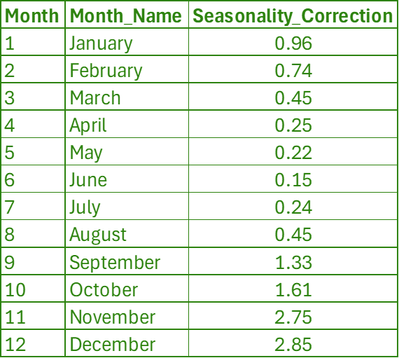
The result is a compact index table that captures how each calendar month systematically deviates from a “typical” month, based on four years of historical data.

How to Read It

In the Fashion4Seasons example, the index tells us how each month typically performs relative to a “normal” month.

On average:

• December, the strongest month, delivers sales 19% above the yearly monthly average.
• February, one of the weakest months, reaches only 84% of the yearly monthly average.

In other words, a raw sales figure observed in December is naturally inflated by seasonality, while the same figure in February is structurally suppressed.

How to Implement It in Analysis or Modeling

To remove this seasonal distortion, we adjust observed sales using the inverse of the seasonality factor.

By multiplying actual sales by (1 / sn.Seasonality_Correction), we effectively strip out the time-of-year effect. What remains is a seasonally neutralized signal - a view of performance driven by the product, campaign, or customer behavior itself, rather than the calendar.

This adjusted metric can then be used consistently:

• for fair MoM or YoY comparisons,
• as an input feature in predictive models, or
• to isolate true campaign impact from seasonal lift.

Let’s implement it for fair MoM comparison:

WITH seasonalitycorrection AS (
    WITH rawtable AS (
        SELECT
            EXTRACT(YEAR FROM fc.DayDate) AS Year_Clean,
            EXTRACT(MONTH FROM fc.DayDate) AS Month_Clean,
            SUM(Sales_USD) AS Sales_USD
        FROM Fact_Sales AS fc
        LEFT JOIN Item_Categories AS ic ON fc.Item_ID = ic.Item_ID
        WHERE ic.Item_Category = 'Winter_Clothing'
          AND EXTRACT(YEAR FROM fc.DayDate) BETWEEN 2020 AND 2023
        GROUP BY 1, 2
    ),
    aggtable AS (
        SELECT
            Month_Clean,
            Sales_USD / AVG(Sales_USD) OVER (PARTITION BY Year_Clean) AS Pct_From_Year_Average
        FROM rawtable
    )
    SELECT
        Month_Clean,
        FORMAT_DATE('%B', DATE(2000, Month_Clean, 1)) AS Month_Name,
        AVG(Pct_From_Year_Average) AS Seasonality_Correction
    FROM aggtable
    GROUP BY 1
    ORDER BY 1
),
monthly_technicolor_down_coat_sales AS (
    SELECT
        FORMAT_DATE('%Y-%m-%d', DATE_TRUNC(fc.DayDate, MONTH)) AS Year_Month,
        EXTRACT(MONTH FROM fc.DayDate) AS Month_Clean,
        SUM(Sales_USD) AS TDC_Sales_USD
    FROM Fact_Sales AS fc
    LEFT JOIN Item_Categories AS ic ON fc.Item_ID = ic.Item_ID
    WHERE Item_Category = 'Technicolor Down Coat'
    GROUP BY 1, 2
),
base AS (
    SELECT
        mtds.Year_Month,
        mtds.TDC_Sales_USD,
        sn.Seasonality_Correction,
        mtds.TDC_Sales_USD
            * SAFE_DIVIDE(1, sn.Seasonality_Correction)
            AS TDC_Sales_SC
    FROM monthly_technicolor_down_coat_sales mtds
    LEFT JOIN seasonalitycorrection sn
        ON mtds.Month_Clean = sn.Month_Clean
    WHERE mtds.TDC_Sales_USD IS NOT NULL
),
lags AS (
    SELECT
        *,
        LAG(TDC_Sales_USD) OVER (ORDER BY Year_Month) AS Prev_Month_Sales,
        LAG(TDC_Sales_SC)  OVER (ORDER BY Year_Month) AS Prev_Month_Sales_SC
    FROM base
)
SELECT
    Year_Month,
    TDC_Sales_USD,
    Seasonality_Correction,
    TDC_Sales_SC,
    SAFE_DIVIDE(
        TDC_Sales_USD - Prev_Month_Sales,
        Prev_Month_Sales
    ) AS MoM,
    SAFE_DIVIDE(
        TDC_Sales_SC - Prev_Month_Sales_SC,
        Prev_Month_Sales_SC
    ) AS SC_Adjusted_MoM
FROM lags
ORDER BY Year_Month DESC;

The output:

From the table above, we can see that despite the strong nominal month-over-month growth from October to November, the increase still falls short of what is typically observed during these months in the winter-clothing category.

Either the Eurodance campaign failed to resonate with the otherwise refined Technicolor Down Coat collection, or this magnificent piece of outerwear was simply ahead of its time… or, quite possibly, both.

The natural next step is to evaluate the adjusted YoY performance of the entire winter-clothing section. It may well be that - when compared to last year’s “urban minimalist” palettes - the new collection actually performed strongly, despite the underwhelming Eurodance campaign.

Can you build that query?

Conclusion

Seasonality Correction offers a pragmatic alternative. By anchoring performance to a stable, multi-year seasonal baseline, it allows analysts to separate what the calendar explains from what the business actually controls. The result is not a more complex model, but a more honest one.

Most importantly, this approach scales. It works just as well for campaign evaluation as it does for feature engineering in predictive models, early performance assessment of new products, or fast decision-making cycles where waiting a full year is not an option.

The real shift is not technical - it’s conceptual. Stop asking whether performance is up or down. Start asking whether it is better or worse than seasonality would predict. That is where signal begins, and noise ends.

---

Originally published on Medium.